Learning Gaits for Unipedal Locomotion
Table of Contents
Overview
The goal of this project is to build a unipedal simulator, based on the 3D One-Leg Hopper from the MIT Leg Lab, which learns to hop (walk/run) in an emulated physical environment using Reinforcement Learning.
We modeled several differently shaped rigid-bodied hoppers within a planar environment with gravity, developed a rendering system to display the unipedal motion in real-time, and implemented a reinforcement learning algorithm to enable our uniped to learn how to walk using various different body models.
Objectives
Implement a working reinforcement learning algorithm that enables the uniped to learn gaits for its locomotion without being given a hard-coded controller for its modeled body.
Physics Engine and Visualization
Our first main goal is to create the the physics simulator and graphics environment to display the uniped virtually. This goal has the following components:
- Physics simulator with capabilities of modeling the following:
- Gravity
- Rigid Body Dynamics
- Prismatic and Revolute Joints
- Collisions/Constrained Dynamics
- Graphics component must be able to render the following:
- Display ground
- Rigid bodies and joints (i.e. the uniped)
- Critical system information (e.g. distance traveled, current epoch, etc.)
Reinforcement Learning
The second major goal of this project is to have a reinforcement learning algorithm that learns a control scheme within the virtual system that we have created. The reinforcement learning component of this project will have the following functionality:
- Effectively learn gaits for unipedal motion
- Send control commands to object model
- Receive reward and state back from the system
- Save controller state (i.e. the rules that the controller is using at any given point in the learning process)
Implementation
In this section, we will discuss the implementation of each of the modules discussed in the previous section. While each of these modules will likely all be run on the same machine, we have the flexibility of running each of the modules on separate machines all connected to the same network.
Physics Engine
After facing several setbacks due to the speed of our custom physics engine and the difficulty of integrating our system across many different programming languages, we decided to use an existing open-source, python-portable engine called Box2D.
This engine meets all the requirements we had in mind. Additionally, since it has been ported to python, we do not have to deal with the architectural difficulty that is involved with interfacing between multiple languages.
In addition, we created the interface to the physics simulation and robot controls using OpenAI Gym's environment object specification. That is, the physics engine can be addressed using the same function calls as OpenAI Gym's existing environments. We chose to do this to increase the portability of our code and make it easy for other reinforcement learning researchers to potentially interact with our project.
Visualization
For the visualization, we used an open-source python wrapper around SDL called PyGame. Since SDL itself is a wrapper around OpenGL, and since PyGame also includes its own windowing capabilities, this allowed us to easily render circles, polygons, lines, and textures onto the screen.
Additionally, SDL provides PyGame with a wrapper around system calls to listen for user events such as keypresses and mouse clicks. This enabled us to create an interactive demonstration for people to attempt to make the unipeds walk with keyboard-based controls.
Reinforcement Learning
The reinforcement learning module (the robot controller) is implemented in Python, using TensorFlow and numpy. Additionally, as mentioned previously, we implemented the interface defined by OpenAI Gym to interact with our custom environment.
The deep Q-learning algorithm itself was written by hand, although its underlying model, a feed-forward, fully connected neural network, was implemented using TensorFlow.
We saved learned policies for later replay by recording the structure and all the learned weights in the neural net.
Outcomes
We successfully set up an envirionment with visualization for several different robot models, which we trained to walk using reinforcement learning. Not all models were successful at this task, and the best learned controllers tended to only take a few steps before falling. We attempted to correct this using different underlying neural net architectures, varying learning rates and learning rate decays, varying amounts of randomness in selecting initial actions, different reward functions, and random initializations.
The network architectures we used were all feed-forward and fully connected, and used between one and four hidden layers, each with 20 to 4096 perceptrons. The larger networks were only used for more complex models like the muscle-constrained kangaroo hopper, which had an action space of size 243. The two-layer model with 20 perceptrons per layer performed relatively well for the simplest models such as the pogo hopper, while none of the models we tried seemed to work exceptionally well with the most complex model, the muscle-constrained kangaroo hopper.
For the learning rates, we tried values between 0.1 and 0.000001, with no decay, linear decay, and exponential decay with decay rates between 0.95 and 0.999. The exponential decay with an initial learning rate of 0.1 to 0.01 was appropriate in most situations.
Additionally, in order to explore the state space more at the beginning of learning, we used an epsilon-greedy approach with an epsilon that decayed over time as the neural net learned a better policy. We initialized epsilon as 1.0 so the initial steps were almost completely random in order to try to explore more possible state-action pairs. We tried both linear and exponential decays, with decay rates between 0.96 and 0.999. Slower decay tended to work well with more complex models since they had larger action spaces to explore.
For the reward function, we always gave a large negative reward when the robot body and/or head contacted the ground, and tried several different schemes for positive rewards. We tried a linearly increasing and cubicly increasing reward as a function of x-distance of the robot from the start position. We tried body position, foot position, and average of body and foot position as the measured x-distance, and found that using the body's x-distance tended to give better results. Using a cubic function was also an attempt to encourage the robot to go further in the x-direction instead of falling forwards at the beginning and gaining a very small reward. In addition to x-distance rewards, we also tried y-distance rewards to encourage the robot to hop vertically, foot-robot x-distance differences to encourage the robot to keep the foot under the head instead of to the side of it, and time-based rewards to encourage the robot to simply stay 'alive' longer, which we believed it would do by hopping more instead of falling. We also tried using a delta-based approach for the measured distances instead of an absolute distance, meaning that the reward was based on the difference between the previous state's x or y and the current x or y instead of the initial state's x or y and the current x or y. The simplest reward function, the linear x-distance from start, tended to give the best results for most models.
Finally, we also tried random initializations, which involved randomly applying actions and translating the robot vertically so it was not touching the ground at initialization. The idea behind this was to learn a larger state space and prevent overfitting to the default initial state of the robot, which had all components vertically aligned, and the robot itself hovering slightly above the ground. However, this actually resulted in worse performance, mostly because the majority of the random states were bad states that the robot would not be able to recover from anyways, so the learned models with random initialization often involved excessive spinning of the body in an attempt to correct the orientation of the robot.
Additionally, states were represented as a vector of concatenated x, y, theta coordinates for every body of the robot, shifted in x so that the robot body's x-position was always 0. This shift was introduced to reduce the size of the state space.
The video below shows some of the outcomes we achieved.
Demo Video
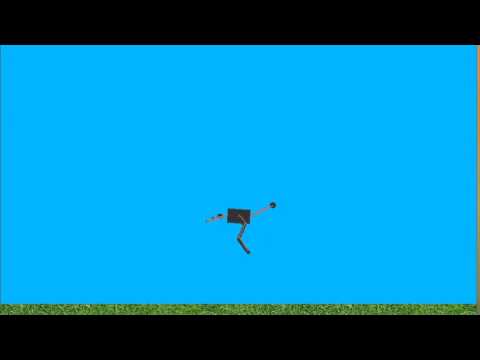
In the first clip of the video, we trained the kangaroo hopper with a time-based and distance-based reward. It learned to sit on one of its legs to maximize the time reward, occasionally scooting forwards to increase its distance reward. This demonstrates the importance of having a good reward function to prevent undesired behavior such as sitting on the ground. The remaining clips do not have time-based rewards.
The second clip shows the pogo hopper learning to take a few steps and go in the correct direction.
After this, we used a more complex model so the robot was able to balance itself by means other than spinning its body.
The clip after that shows random initialization with the pogo hopper. Notice that the initial position is usually of very poor quality, often with the foot starting above the head or to the side of it.
Next is the more complex robot with muscle constraints. Unfortunately, it did not learn a very good policy, most likely because the size of the action space is too large and the robot was not trained for a sufficient amount of time.
If we were to redo this project or if we simply had more time, we would try different architectures, such as deeper networks or even recurrent models. Additionally, we might use each 'step' as the unit for an epoch instead of each trial (initialization time to time when we detect a collision between the ground and body and/or head). This would allow us to give a greater reward for the entire sequence of events that went into taking a step, and a smaller reward for the sequence of events that lead to a failure mode. Additionally, we would try different combinations of hyperparameters to optimize how well our models work.